 Superior Courts Act, 2013
R 385
Mine Health and Safety Act, 1996 (Act No. 29 of 1996)RegulationsGuideline for a Mandatory Code of PracticeOccupational Health Programme (Occupational Hygiene and Medical Surveillance) on Personal Exposure to Airborne PollutantsAnnexuresAnnexure B : HEG determination, example of statistical approach |
(This Annexure is attached for information purposes only)
Introductory information:
1In statistics, a confidence interval is a particular kind of interval estimate of a population parameter. Instead of estimating the parameter by a single value, an interval likely to include the parameter is given. Thus, confidence intervals are used to indicate the reliability of an estimate. How likely the interval is to contain the parameter is determined by the confidence level or confidence coefficient. Increasing the desired confidence level will widen the confidence interval.
A confidence interval is always qualified by a particular confidence level, usually expressed as a percentage. The end points of the confidence interval are referred to as confidence limits.
1 Interval estimation [online] available from https:llen.wikipedia.orglwiki/Interval_estimation
Step 1
Action to be performed:
| 1. | Capture sampling data in Microsoft Excel,. |
| 2. | Determine the descriptive statistics for the data by utilising Microsoft Excel Analysis ToolPak, |
To install the Analysis ToolPak:
| • | On the Tools menu, select Add-Ins. |
| • | If Analysis ToolPak is not listed in the Add-Ins dialog box, click Browse and locate the drive, folder name and file name for the Analysis ToolPak Add-Ins, Analys32.xll usually located in the Library/Analysis folder, or run the Setup program if it is not installed. |
| • | Select the Analysis ToolPak check box. |
To use the Analysis ToolPak:
| • | Before using the Analysis ToolPak, you must first arrange the data you want to analyse in one column (e.g. A1 to A40 - if you have 40 values that you want to analyse). |
| • | On the Tools menu, click Data Analysis. |
| • | In the Analysis Tools box, select the Descriptive Statistics tool. |
| • | Enter the input range (e.g. A1 to A40). |
| • | Select the Grouped by Columns option. |
| • | Select the output range (e.g. B1 to B40). |
| • | Select the Summary Statistics option. |
| • | Select the Confidence Level of Mean option and enter this value as being 95%. |
| • | Select OK. |
Expected result:
|
Example of data entered into Microsoft Excel |
Expected result after completing actions as indicated under STEP 1 |
|
|
DATA |
DESCRIPTIVE STATISTICS |
|
|
1.78 |
Mean |
1.963 |
|
1.87 |
Standard error |
0.148 |
|
2.15 |
Median |
2.150 |
|
2.29 |
Mode |
#N/A |
|
2.54 |
Standard deviation |
0.535 |
|
1.51 |
Sample variance |
0.286 |
|
2.47 |
Kurtosis |
-0.665 |
|
2.45 |
Skewness |
-0.689 |
|
1.32 |
Range |
1.65 |
|
2.32 |
Minimum |
0.89 |
|
2.48 |
Maximum |
2.54 |
|
1.45 |
Sum |
25.52 |
|
0.89 |
Count |
13 |
|
|
Confidence level (95.0%) |
0.323 |
Step 2
Action to be performed:
From the descriptive statistics calculate the following:
|
(A) 2SD |
= 2 x Standard Deviation |
e.g. 2 x 0.535 = 1.071 |
|
(B) Mean - 2SD |
= Mean - 2SD |
e.g. 1.963 - 1.071 = 0.892 |
|
(C) Mean + 2SD |
= Mean - 2SD |
e.g. 1.964 + 1.071 = 3.034 |
|
(D) 90th Percentile value by utilizing the following Microsoft Excel formulae: |
||
= PERCENTILE (A1:A40,0.9) = 2.478 (for the data used in this example)
where:
"A1:A40" = Range were data is entered in Microsoft Excel spread sheet
"0,9" = The percentile to be calculated, in this case the 90th percentile
Interpretation:
From the calculation performed above it can already be estimated that this HEG in NOT statistically correct defined, as:
| • | The mean value falls within the "B Category and the 90th percentile value falls within the "A Category". For a HEG to be statistically correctly defined its mean and 90th percentile values will almost always fall within the same classification band. |
Step 3
Action to be performed:
Determine if 95% of the samples taken falls within two standard deviations (2SD) form the mean value.
Example:
| • | 95% of the samples must be between "Mean - 2SD" (0.892) and "Mean + 2SD" (3.034) |
| • | From the data 1 sample (0.59) is smaller than "Mean 2SD" and O samples are larger than Mean .+ 2SD". |
Interpretation:
One out of 13 samples represent 7.69 % of the sample group (e.g. 1/13 x 100 = 7.69%).
This is more than the allowable 5% and therefore the HEG cannot be seen as statistically correctly defined.
Step 4
Action to be performed:
Draw a histogram to graphically indicate the data.
Expected result:
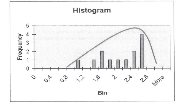
Interpretation:
From the histogram, it is also clear that the HEG is NOT statistically correctly defined (no bell curve). Only two things can be done to correct this situation:
| • | Obtain more samples to determine the correct distribution of samples within the HEG. This is currently being forced by the legislated sampling strategy as the "mean" value reported for dose (concentration of airborne pollutant(s) to which a person is exposed) allocations, (for an OEL of two in this example) falls within a "B Category" (5% sampled over six months) but the 90th percentile value is reported as an "A Category thus forcing more samples to be taken (5% over three MTh's). |
| • | Conduct an investigation to determine if more than one HEG is being represented by the data. |
Step 5
Action to be performed:
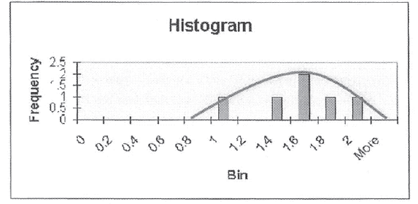
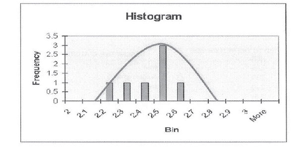
Conduct an investigation to determine if more than one HEG is being represented by the data. This can be done by investigation and following the methodology as explained, up to this point (for example):
After investigation, the HEG was divided into two separate HEGs (intake-side HEG and return-side HEG).
The data collected was then allocated to the two HEGs and the statistical analysis revealed the following:
|
DATA ALLOCATED TO THE INTAKE SIDE HEG |
DESCRIPTIVE STATISTICS |
|
|
0.89 |
Mean |
1.47 |
|
1.32 |
Standard error |
0.14 |
|
1.78 |
Median |
1.48 |
|
1.87 |
Mode |
#N/A |
|
1.51 |
Standard deviation |
0.35 |
|
1.45 |
Sample variance |
0.12 |
|
|
Kurtosis |
0.57 |
|
|
Skewness |
-0.72 |
|
|
Range |
0.98 |
|
|
Minimum |
0.89 |
|
|
Maximum |
1.87 |
|
|
Sum |
8.82 |
|
|
Count |
6 |
|
|
Confidence level (95.0%) |
0.36 |
CALCULATIONS
| 2 X SD | = 0.702 |
| Mean - 2SD | = 0.767 |
| Mean + 2SD | = 2.172 |
| 90th percentile | = 1.825 |
Interpretation:
From the above it can already be estimated that this HEG is statistically correctly defined, as the mean value (1.47) falls within the "B Category' and the 90th percentile value (1.825) also falls within the "B Category".
DOES 95% OF THE SAMPLES FALL WITHIN TWO STANDARD DEVIATIONS (SD) FROM THE MEAN?
| (A) | 95% of the samples must be between mean - 2SD (0.7674) and mean + 2SD (2.173) |
| (B) | From "DATA": 0 sample < mean - 2SD0 samples > Mean 2SD |
| (C) | 0/6 = 0% |
This is within the allowable 5% and therefore the HEG is statistically correctly defined.
|
DATA ALLOCATED TO THE RETURN SIDE |
DESCRIPTIVE STATISTICS |
|
|
HEG |
||
|
2.15 |
Mean |
2.38 |
|
2.29 |
Standard error |
0.05 |
|
2.32 |
Median |
2.45 |
|
2.54 |
Mode |
#N/A |
|
2.47 |
Standard deviation |
0.13 |
|
2.45 |
Sample variance |
0.01 |
|
2.48 |
Kurtosis |
-0.26 |
|
|
Skewness |
-0.80 |
|
|
Range |
0.39 |
|
|
Minimum |
2.15 |
|
|
Maximum |
2.54 |
|
|
Sum |
16.7 |
|
|
Count |
7 |
|
|
Confidence level (95.0%) |
0.12 |
CALCULATIONS
2 X SD = 0.274434
Mean - 2SD = -2.11128
Mean + 2SD = 2.660149
90th percentile = 2.504
Interpretation:
From the above it can already be estimated that this HEG is statistically correctly defined, as the mean value (2.39) falls within the "A Category" and the 90th percentile value (2.504) also falls within the "A Category".
DOES 95% OF THE SAMPLES FALL WITHIN TWO STANDARD DEVIATIONS (SD) FROM THE MEAN?
(A) 95% of the samples must be between mean - 2SD (-2.514) and mean + 2SD (7.286)
(B) From "DATA": 0 sample < mean - 2SD and 0 samples > mean + 2SD
| (C) | 0/7 = 0%. This is within the allowable 5% and therefore the HEG is statistically correctly defined. |
Step 6 - Paired T-test